A simple illustration of a novel technique called Integrated Gradients to quantify & visualize feature importance in neural networks regardless of model architecture. Implementation of ideas from the paper Axiomatic Attribution for Deep Networks on text data.

Background
Deep neural networks are notorious for not being explainable. Integrated Gradients, a method proposed in the aforementioned paper, is a very easy and fast method to understand feature importance and are not dependent on model architecture.
Key Idea
If we linearly interpolate our input sample from an appropriately chosen baseline with small increments, and sum the gradients of the output prediction w.r.t inputs of each interpolation, the resulting sum would represent the attributions (importance) of input features.
Code Walkthrough
For full code, refer to the Google Colab
Step 1: Build a model
Download the dataset. Here we are using the ag_news_subset dataset. The goal is to predict the topic (out of 4 possible classes) given a news headline. We build a simple Bi-Directional LSTM model, which would give us about 85% accuracy after 5 epochs of training.
Model: "sequential" _________________________________________________________________
Layer (type)                 Output Shape              Param #    ================================================================= embedding (Embedding)        (None, None, 64)          64000      _________________________________________________________________ bidirectional (Bidirectional (None, 64)                24832      _________________________________________________________________
dense (Dense)                (None, 16)                1040       _________________________________________________________________
probs (Dense)                (None, 4)                 68         =================================================================
Total params: 89,940
Trainable params: 89,940
Non-trainable params: 0
Step 2: Integrated Gradients
Since, the embedding layer in TensorFlow is non-differentiable, we will create a slice of the model comprising of all the layers after the embedding layer.
embed_layer = model.get_layer('embedding')

# build new model with all layers after embedding layer
new_model = tf.keras.Sequential()
for layer in model.layers[1:]:
    new_model.add(layer)
To calculate integrated gradients for a given sample, first we need to select a baseline. The paper suggests using a zero embedding vector.
# get embeddings
sample_embed = embed_layer(sample_vector)

# Create a Baseline vector with zero embeddings
baseline_embed = tf.zeros(shape=tf.shape(sample_embed))
Linearly interpolate from baseline vector to the sample vector.
def interpolate_texts(baseline, vector, m_steps):

    """ Linearly interpolate the sample vector
    (embedding layer output)"""

    # Generate m_steps intervals for integral_approximation() below.
    alphas = tf.linspace(start=0.0, stop=1.0, num=m_steps+1)
    alphas_x = alphas[:, tf.newaxis, tf.newaxis]
    delta = vector - baseline
    texts = baseline + alphas_x * delta
    return texts


n_steps = 50


interpolated_texts = interpolate_texts(baseline_embed,
                                       sample_embed,
                                       n_steps)
Now, compute gradients of the model output for the interpolated vectors w.r.t the vectors, and particularly the prediction index of the true class. We can use this index to understand misclassified samples as well. Scroll down for more on this.
def compute_gradients(t, target_class_idx):

    """ compute the gradient wrt to embedding layer output """

    with tf.GradientTape() as tape:
        tape.watch(t)
        probs = new_model(t)[:, target_class_idx]
    grads = tape.gradient(probs, t)
    return grads

# sample label is the true class of the sample
path_gradients = compute_gradients(interpolated_texts, sample_label)
Sum up all the gradients, normalize by number of steps and multiply by the difference of sample vector and baseline vector (remember baseline vector was chosen to be a vector of zeros).
# sum the grads of the interpolated vectors
all_grads = tf.reduce_sum(path_gradients, axis=0) / n_steps
# mulitply grads by (input - baseline); baseline is zero vectors
x_grads = tf.math.multiply(all_grads, sample_embed)
# sum all gradients across the embedding dimension
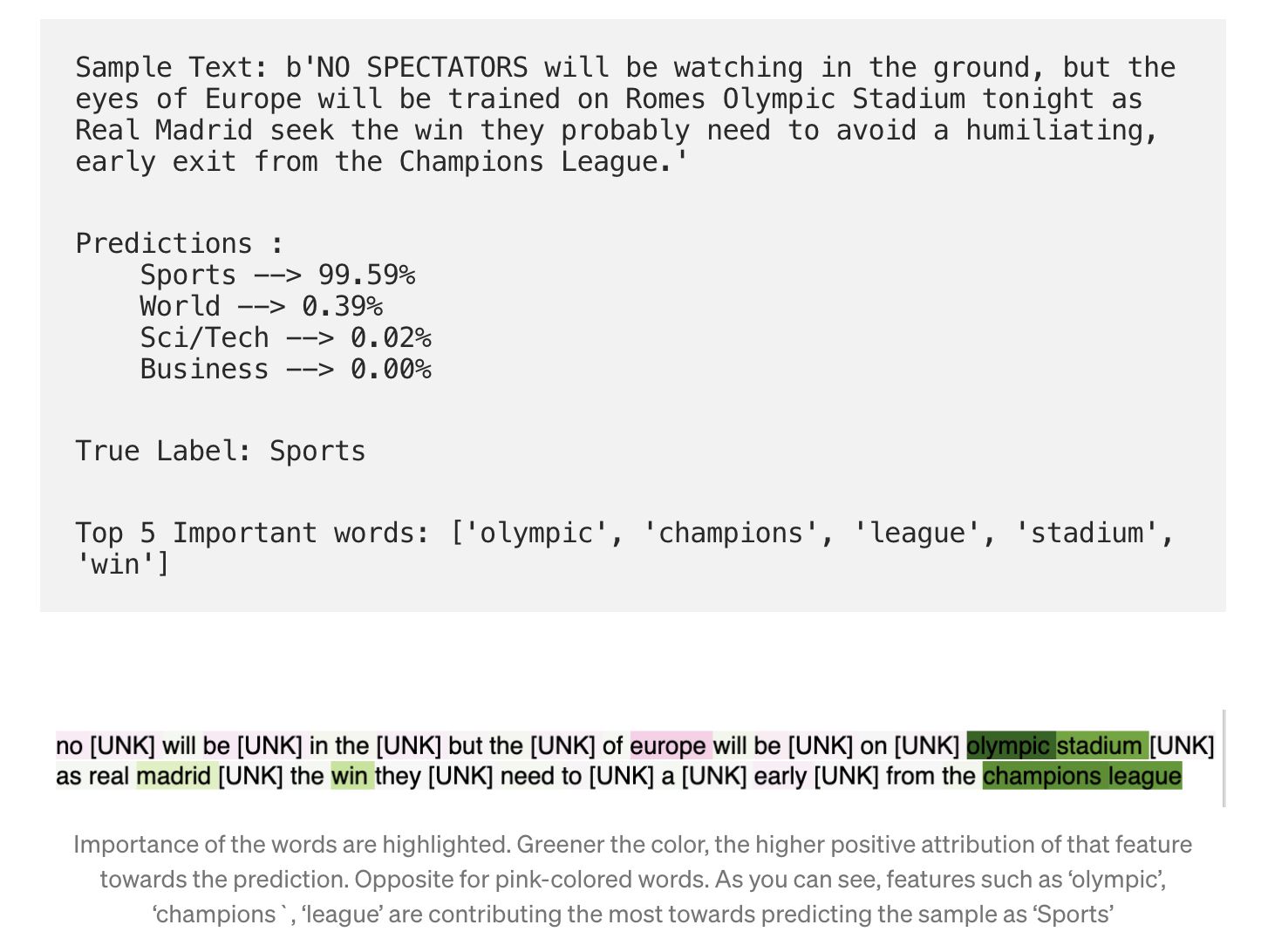
igs = tf.reduce_sum(x_grads, axis=-1).numpy()Step 3: Visualize the output
Another example where the model misclassified.
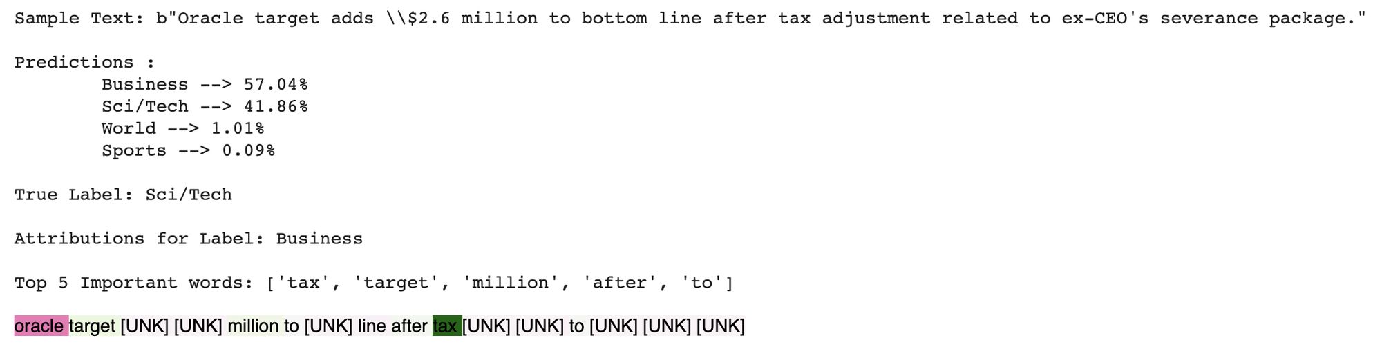
Sci/Tech but the model predicts Business. As you can see, it does so while focusing (attributing positively more on) the word tax and negatively attributing to the word Oracle. 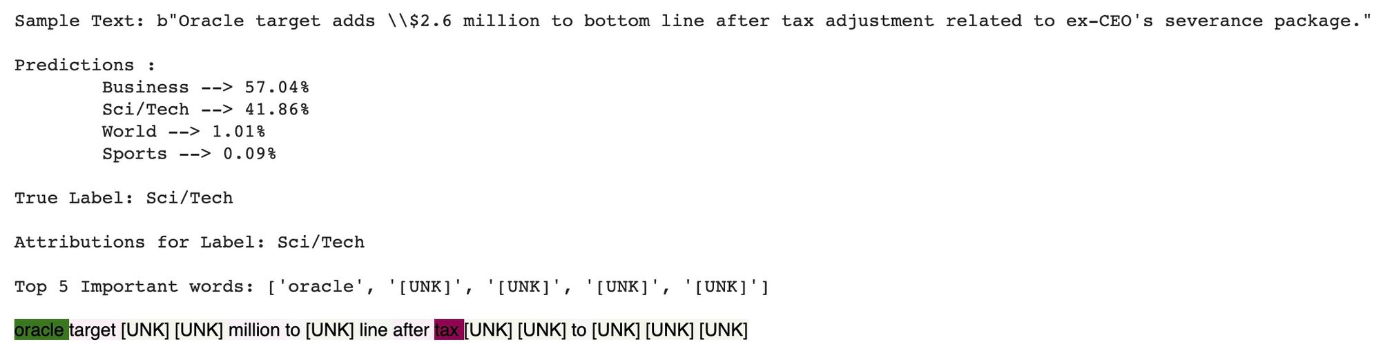
Sci/Tech, the attributions are totally reversed. Lessons: We can may be take a look at all the samples with Oracle in them and see if they are heavily biased towards Sci/Tech leading the model to disassociate the word Oracle from BusinessApplications at Asurion
At Asurion, we build state-of-the-art neural networks for various business critical applications such as customer experience / churn prediction using textual data where explainability is critical to drive business decisions, product development and stakeholder partnership. We continue to apply novel ideas and technologies to deliver the fastest and convenient solutions that enable, support and protect people's tech products and digital life.